Everyone interested in computer graphics knows that geometry transformation is basically a set of vector multiplications by some matrix, but have you ever wondered what this matrix actually contains? Have you ever try to visually interpret it? This episode will try to put some light on this subject.
Linear Combination
Linear Combination is a very general concept. Basically, if you have a set of vectors and set of scalars and you sum the multiplication of each vector by each scalar, you get a vector that you can call a linear combination of this set.

Standard Basis Vectors
Although this term might sound complicated, it really isn’t – standard basis vectors is a set of unit vectors where each one is pointing in the direction of the axes of some Cartesian coordinate system. For example, in case of standard Cartesian 3D space, the basis vectors would be:

One of the most important properties about vectors is that every vector is a linear combination of standard basis vectors. This is represented by the equation below.

Although it sounds obvious it has some interesting implications. Here’s a picture to better portray this concept.
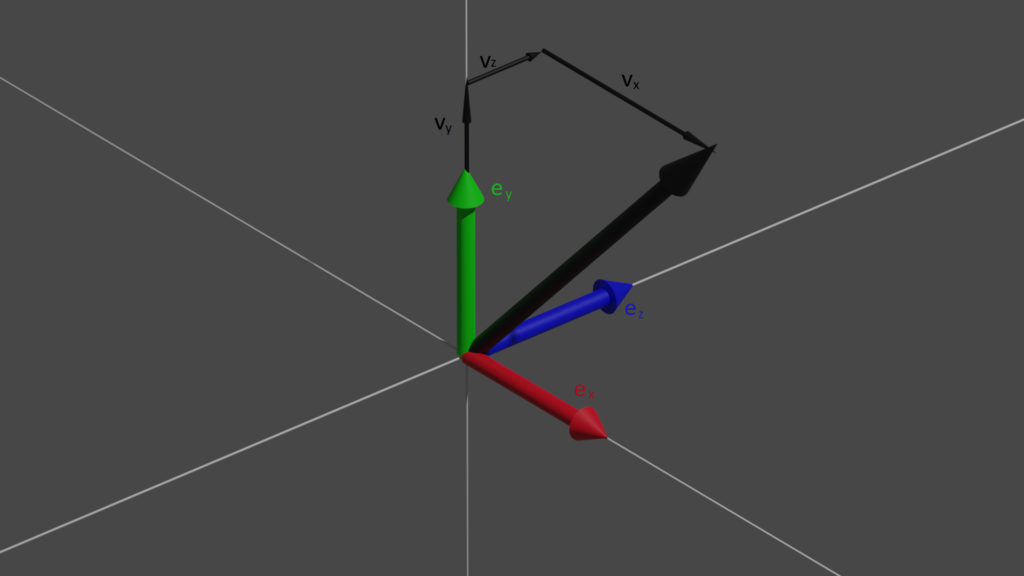
The black vector can has three components and in order to build this vector, we can multiply each of this component by a corresponding basis vector and then add them together. Note that thin black vectors are actually a resulting vector of multiplying given basis vector by a corresponding component (scalar) and not the component itself.
Vector and Matrix Multiplication
So far you’ve learnt one interesting thing about linear combination and one obvious thing about standard basis vectors, but why would you ever want that? This is all to help you understand why almost every geometrical transformation is a multiplication by a matrix and what this matrix actually contain. In my personal opinion, this is the most important thing to remember when learning geometrical transformation and make every other thing very easy to understand.
First, let’s try to multiply all of our standard basis vectors by some matrix.


The conclusion is that each row in this matrix holds a result of matrix multiplication by a standard basis vector. Now let’s try to put our knowledge into use. We know that every vector can be written as a linear combination of its components and basis vectors.

We know that multiplication has associative property (A(BC) = (AB)C) and distributive property ((A+B)C = AC + BC), so we can rewrite this equation like this.

And now it is simple – we know that when we multiply our matrix by a base vector, we get a single row from it, so this equation unrolls to:

And there we go – the result of a vector and matrix multiplication is a linear combination of the rows of the matrix and a vector. The key is to interpret those rows as basis vectors.
Application
Just for fun, lets construct a matrix that will allow us to scale a mesh over an x-axis. For better visualization, let’s look at the following pictures.
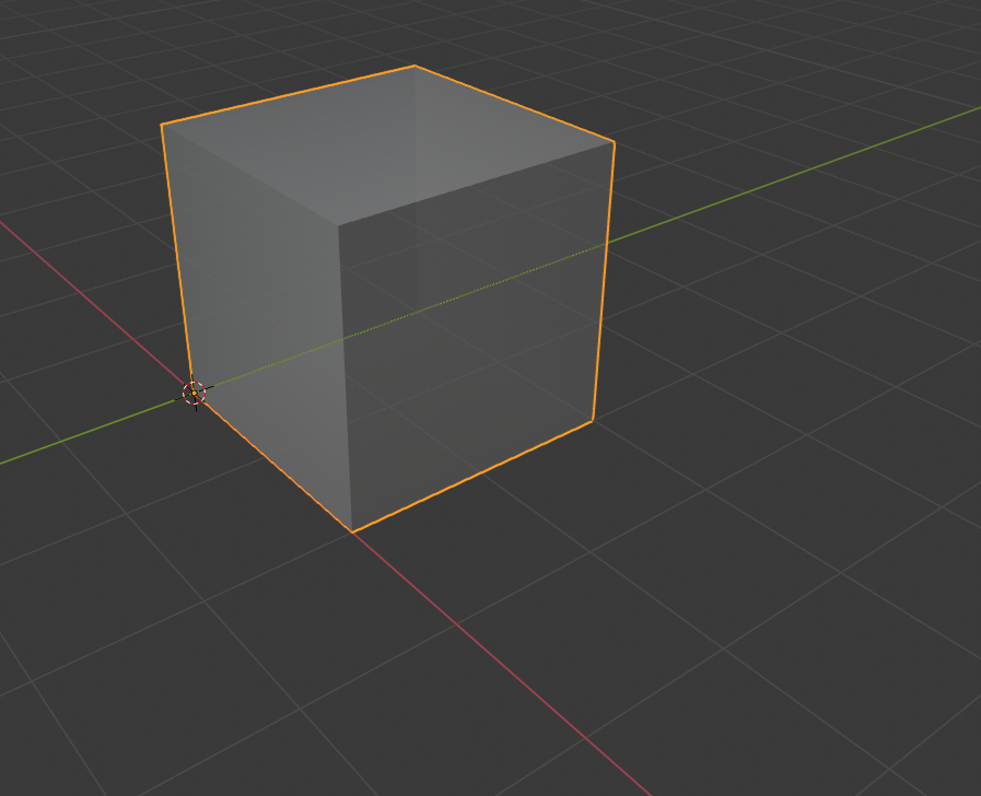
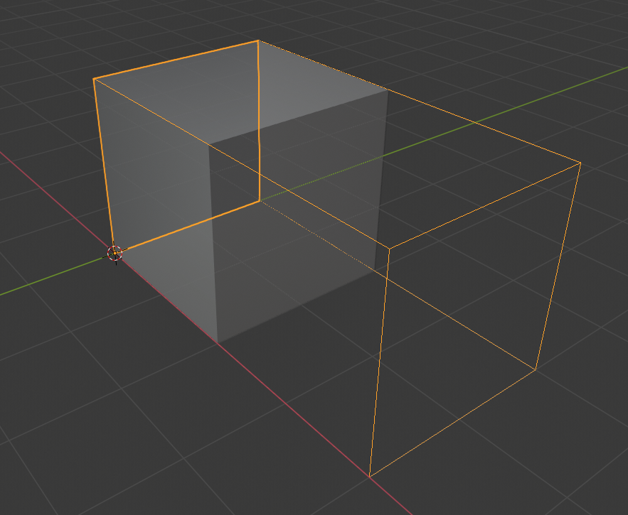
On the left side we see original cube – docked at the point of origin and on the right side we see the resulting cube – scaled over x-axis by a factor of two. If we look at the global positions, we can see that in order to do that, we need to multiply every x-component of each vector by 2. For example, if we take one of the bottom vertices, originally it had position (2, 0, 0) and after the transformation it has the position (4, 0, 0) and (2, 0, 2) would be (4, 0, 2).
In order to achieve this, we need to multiply the x-axis vector by a factor of 2 while the other by a factor of 1. Lets put this all in our equation.

If we would then like to describe this transformation with a matrix, we will get this.

Now imagine if you would like to scale entire object by half in every direction – can you imagine how the transformation matrix would look like? I hope so! And just as easy as deconstructing a matrix with this knowledge is, same goes with constructing one. Simply think of what you transformation does to basis vectors and then put them into corresponding row of a matrix. Good luck and see you in the next episode!
Leave a Reply